Statistics and machine learning approaches

A couple of years back, I was part of a team that delivered a workshop in machine learning. Given my background, I had been asked to do a half-day session on Regression, and was told that the standard software package being used was the scikit-learn package in python.

Both the programming language and the package were new to me, so I dug around a few days before the workshop, trying to figure out regression. Despite my best efforts, I couldn’t locate how to find out the R^2. What some googling told me was surprising:

There exists no R type regression summary report in sklearn. The main reason is that sklearn is used for predictive modelling / machine learning and the evaluation criteria are based on performance on previously unseen data

As it happened, I requested the students at the workshop to install a package called statsmodels, which provides standard regression outputs. And then I proceeded to lecture to them on regression as I know it, including significance scores, p values, t statistics, multicollinearity and the likes. It was only much later was I to figure out that that is now how regression (and logistic regression) is done in the machine learning world.

In a statistical framework, the data sets in regression are typically “long” – you have a large number of data points, and a small number of variables. Putting it differently, we start off with a model with few degrees of freedom, and then “constrain” the variables with a large enough number of data points, so that if a signal exists, and it is in the right format (linear relationship and all that), we can pin it down effectively.

In a machine learning framework, it is common to run a regression where the number of data points is of the same order of magnitude as, or even smaller than the number of variables. Strictly speaking, such a problem is unbounded (there are too many degrees of freedom), and so regression is not well-defined. Instead, we rely upon “regularisation methods” to “tie down” the variables and (hopefully) produce a consistent solution.

Moreover, machine learning approaches are common to problems where individual predictor variables don’t have meaning. In this scenario, knowing whether a particular variable is significant or not is of no utility. Then, the signal in machine learning lies in the combination of variables, which means that multicollinearity (correlation between predictor variables) is not really a bad thing as it is in statistics. Variables not having meanings means that there are no correlations per se to be defined, and so machine learning models are harder to interpret, and are more likely to have hidden spurious correlations.

Also, when you have a small number of variables and a large number of data points, it is easy to get an “exact solution” for regression, which is what statistical methods use. In a machine learning framework with “wide” data, though, exact solutions are computationally infeasible, and so you need to use approximate algorithms such as gradient descent – which are common across ML techniques.

All in all, while statistics and machine learning might use techniques with the same name (“regression”, for example), they are both in theory and practice, very different ways to solve the problem. The important thing is to figure out the approach most suited for a particular problem, and use it accordingly.

Statistics and machine learning

So a group of statisticians (from Cyprus and Greece) have written an easy-to-read paper comparing statistical and machine learning methods in time series forecasting, and found that statistical methods do better, both in terms of accuracy and computational complexity.

To me, there’s no surprise in the conclusion, since in the statistical methods, there is some human intelligence involved, in terms of removing seasonality, making the time series stationary and then using statistical methods that have been built specifically for time series forecasting (including some incredibly simple stuff like exponential smoothing).

Machine learning methods, on the other hand, are more general purpose – the same neural networks used for forecasting these time series, with changed parameters, can be used for predicting something else.

In a way, using machine learning for time series forecasting is like using that little screwdriver from a Swiss army knife, rather than a proper screwdriver. Yes, it might do the job, but it’s in general inefficient and not an effective use of resources.

Yet, it is important that this paper has been written since the trend in industry nowadays has been that given cheap computing power, machine learning be used for pretty much any problem, irrespective of whether it is the most appropriate method for doing so. You also see the rise of “machine learning purists” who insist that no human intelligence should “contaminate” these models, and machines should do everything.

By pointing out that statistical techniques are superior at time series forecasting compared to general machine learning techniques, the authors bring to attention that using purpose-built techniques can actually do much better, and that we can build better systems by using a combination of human and machine intelligence.

They also helpfully include this nice picture that summarises what machine learning is good for, and I wholeheartedly agree: 

The paper also has some other gems. A few samples here:

Knowing that a certain sophisticated method is not as accurate as a much simpler one is upsetting from a scientific point of view as the former requires a great deal of academic expertise and ample computer time to be applied.


[…] the post-sample predictions of simple statistical methods were found to be at least as accurate as the sophisticated ones. This finding was furiously objected to by theoretical statisticians [76], who claimed that a simple method being a special case of e.g. ARIMA models, could not be more accurate than the ARIMA one, refusing to accept the empirical evidence proving the opposite.


A problem with the academic ML forecasting literature is that the majority of published studies provide forecasts and claim satisfactory accuracies without comparing them with simple statistical methods or even naive benchmarks. Doing so raises expectations that ML methods provide accurate predictions, but without any empirical proof that this is the case.


At present, the issue of uncertainty has not been included in the research agenda of the ML field, leaving a huge vacuum that must be filled as estimating the uncertainty in future predictions is as important as the forecasts themselves.

Machine learning and degrees of freedom

For starters, machine learning is not magic. It might appear like magic when you see Google Photos automatically tagging all your family members correctly, down to the day of their birth. It might appear so when Siri or Alexa give a perfect response to your request. And the way AlphaZero plays chess is almost human!

But no, machine learning is not magic. I’d made a detailed argument about that in the second edition of my newsletter (subscribe if you haven’t already!).

One way to think of it is that the output of a machine learning model (which could be anything from “does this picture contain a cat?” to “is the speaker speaking in English?”) is the result of a mathematical formula, whose parameters are unknown at the beginning of the exercise.

As the system gets “trained” (of late I’ve avoided using the word “training” in the context of machine learning, preferring to use “calibration” instead. But anyway…), the hitherto unknown parameters of the formula get adjusted in a manner that the formula output matches the given data. Once the system has “seen” enough data, we have a model, which can then be applied on unknown data (I’m completely simplifying it here).

The genius in machine learning comes in setting up mathematical formulae in a way that given input-output pairs of data can be used to adjust the parameters of the formulae. The genius in deep learning, which has been the rage this decade, for example, comes from a 30-year old mathematical breakthrough called “back propagation”. The reason it took until a few years back for it to become a “thing” has to do with data availability, and compute power (check this terrific piece in the MIT Tech Review about deep learning).

Within machine learning, the degree of complexity of a model can vary significantly. In an ordinary univariate least squares regression, for example, there are only two parameters the system can play with (slope and intercept of the regression line). Even a simple “shallow” neural network, on the other hand, has thousands of parameters.

Because a regression has so few parameters, the kind of patterns that the system can detect is rather limited (whatever you do, the system can only draw a line. Nothing more!). Thus, regression is applied only when you know that the relationship that exists is simple (and linear), or when you are trying to force-fit a linear model.

The upside of simple models such as regression is that because there are so few parameters to be adjusted, you need relatively few data points in order to adjust them to the required degree of accuracy.

As models get more and more complicated, the number of parameters increases, thus increasing the complexity of patterns that can be detected by the system. Close to one extreme, you have systems that see lots of current pictures of you and then identify you in your baby pictures.

Such complicated patterns can be identified because the system parameters have lots of degrees of freedom. The downside, of course, is that because the parameters start off having so much freedom, it takes that much more data to “tie them down”. The reason Google Photos can tag you in your baby pictures is partly down to the quantum of image data that Google has, which does an effective job of tying down the parameters. Google Translate similarly uses large repositories of multi-lingual text in order to “learn languages”.

Like most other things in life, machine learning also involves a tradeoff. It is possible for systems to identify complex patterns, but for that you need to start off with lots of “degrees of freedom”, and then use lots of data to tie down the variables. If your data is small, then you can only afford a small number of parameters, and that limits the complexity of patterns that can be detected.

One way around this, of course, is to use your own human intelligence as a pre-processing step in order to set up parameters in a way that they can be effectively tuned by data. Gopi had a nice post recently on “neat learning versus deep learning“, which is relevant in this context.

Finally, there is the issue of spurious correlations. Because machine learning systems are basically mathematical formulae designed to learn patterns from data, spurious correlations in the input dataset can lead to the system learning random things, which can hamper its predictive power.

Data sets, especially ones that have lots of dimensions, can display correlations that appear at random, but if the input dataset shows enough of these correlations, the system will “learn” them as a pattern, and try to use them in predictions. And the more complicated your model gets, the harder it is to know what it is doing, and thus the harder it is to identify these spurious correlations!

And the thing with having too many “free parameters” (lots of degrees of freedom but without enough data to tie down the parameters) is that these free parameters are especially susceptible to learning the spurious correlations – for they have no other job.

Thinking about it, after all, machine learning systems are not human!

JEE coaching and high school learning

One reason I’m not as good at machine learning as I can possibly be is because I suck at linear algebra. I totally completely suck at it. Seven years of usage of R has meant that at least I no longer get spooked out by the very sight of vectors or matrices, and I understand the concept of matrix multiplication (an operator rotating a vector), but I just don’t get linear algebra.

For example, when I see terms such as “singular value decomposition” I almost faint. Multiple repeated attempts at learning the concept have utterly failed. Don’t even get me started on the more complicated stuff – and machine learning is full of them.

My inability to understand linear algebra runs deep, and it’s mainly due to a complete inability to imagine vectors and matrices and matrix operations. As far back as I remember, I have hated matrices and have tried to run away from it.

For a long time, I had placed the blame for this on IIT Madras, whose mathematics department in its infinite wisdom had decided to get its brilliant Graph Theory expert to teach us matrices. Thinking back, though, I remember going in to MA102 (Vectors, Matrices and Differential Equations) already spooked. The rot had set in even earlier – in school.

The problem with class 11 in my school (a fairly high-profile school which was full of studmax characters) was that most people harboured ambitions of going to IIT, and had consequently enrolled themselves in formal coaching “factories”. As a result, these worthies always came to maths, physics and chemistry classes “ahead” of people like me who didn’t go for such classes (I’d decided to chill for a year after a rather hectic class 10 when I’d been under immense pressure to get my school a “centum”).

Because a large majority of the class already knew what was to be taught, teachers had an incentive to slack. Also the fact that most students were studmax had meant that people preferred to mug on their own rather than display their ignorance in class. And so jai happened.

I remember the class when vectors and matrices were introduced (it was in class 11). While I don’t remember too many details, I do remember that a vocal majority already knew about “dot product” and “cross product”. It was similar a few days later when the vocal majority knew matrix multiplication.

And so these concepts were glossed over, and lacking a grounding in fundamentals, I somehow never “got” the concept.

In my year (2000), CBSE decided to change format for its maths examination – everyone had to attempt “Part A” (worth 70 marks) and then had a choice between “Part B” (vectors, matrices, etc.) and “Part C” (introductory statistics). Most science students were expected to opt for Part B (Part C had been introduced for the benefit of commerce students studying maths since they had little to gain from reading about vectors). For me and one other guy from my class, though, it was a rather obvious choice to do Part C.

I remember the invigilator (who was from another school) being positively surprised during my board exam when I mentioned that I was going to attempt Part C instead of Part B. He muttered something to the extent of “isn’t that for commerce students?” but to his credit permitted us to do the paper in whatever way we wanted (I fail to remember why I had to mention to him I was doing Part C – maybe I needed log tables to do that).

Seventeen odd years down the line, I continue to suck at linear algebra and be stud at statistics. And it is all down to the way the two subjects were introduced to me in school (JEE statistics wasn’t up to the same standard as Part C so the school teachers did a great job of teaching that).

Medium stats

So Medium sends me this email:

Congratulations! You are among the top 10% of readers and writers on Medium this year. As a small thank you, we’ve put together some highlights from your 2016.

Now, I hardly use Medium. I’ve maybe written one post there (a long time ago) and read only a little bit (blogs I really like I’ve put on RSS and read on Feedly). So when Medium tells me that I, who considers myself a light user, is “in the top 10%”, they’re really giving away the fact that the quality of usage on their site is pretty bad.

Sometimes it’s bloody easy to see through flattery! People need to be more careful on what the stats they’re putting out really convey!


Horses, Zebras and Bayesian reasoning

David Henderson at Econlog quotes a doctor on a rather interesting and important point, regarding Bayesian priors. He writes:

 Later, when I went to see his partner, my regular doctor, to discuss something else, I mentioned that incident. He smiled and said that one of the most important lessons he learned from one of his teachers in medical school was:

When you hear hooves, think horses, not zebras.

This was after he had some symptoms that are correlated with heart attack and panicked and called his doctor, got treated for gas trouble and was absolutely fine after that.

Our problem is that when we have symptoms that are correlated with something bad, we immediately assume that it’s the bad thing that has happened, and panic. In that process we don’t consider alternate reasonings, and then do a Bayesian analysis.

Let me illustrate with a personal example. Back when I was a schoolboy, and I wouldn’t return home from school at the right time, my mother would panic. This was the time before cellphones, remember, and she would just assume that “the worst” had happened and that I was in trouble somewhere. Calls would go to my father’s office, and he would ask her to wait, though to my credit I was never so late that they had to take any further action.

Now, coming home late from school can happen due to a variety of reasons. Let us eliminate reasons such as wanting to play basketball for a while before returning – since such activities were “usual” and been budgeted for. So let’s assume that there are two possible reasons I’m late – the first is that I had gotten into trouble – I had either been knocked down on my way home or gotten kidnapped. The second is that the BTS (Bangalore Transport Service, as it was then called) schedule had gone completely awry, thanks to which I had missed my usual set of buses, and was thus delayed. Note that me not turning up at home until a certain point of time was a symptom of both of these.

Having noticed such a symptom, my mother would automatically come to the “worst case” conclusion (that I had been knocked down or kidnapped), and panic.   But then I’m not sure that was the more rational reaction. What she should have done was to do a Bayesian analysis and use that to guide her panic.

Let A be the event that I’d been knocked over or kidnapped, and B be the event that the bus schedule had gone awry. Let L(t) be the event that I haven’t gotten home till time t, and that such an event has been “observed”. The question is that, with L(t) having been observed, what are the odds of A and B having happened? Bayes Theorem gives us an answer. The equation is rather simple:

P(A | L(t) ) =  P(A).P(L(t)|A) / (P(A).P(L(t)|A) + P(B).P(L(t)|B) )

P(B|L(t)) is just one minus the above quantity (we assume that there is nothing else that can cause L(t)) .

So now let us give values. I’m too lazy to find the data now, but let’s say we find from the national crime data that the odds of a fifteen-year-old boy being in an accident or kidnapped on a given day is one in a million. And if that happens, then L(t) obviously gets observed. So we have

P(A) = \frac{1}{1000000}
P(L(t) | A) = 1

The BTS was notorious back in the day for its delayed and messed up schedules. So let us assume that P(B) is \frac{1}{100}. Now, P(L(t)|B) is tricky, and the reason the (t) qualifier has been added to L. The larger t is, the smaller the value of L(t)|B. If there is a bus schedule breakdown, there is probably a 50% probability that I’m not home an hour after “usual”. But there is only a 10% probability that I’m not home two hours after “usual” because a bus breakdown happened. So

P(L(1)|B) = 0.5
P(L(2)|B) = 0.1

Now let’s plug in and based on how delayed I was, find the odds that I was knocked down/kidnapped. If I were late by an hour,
P(A|L(1)) = \frac{ \frac{1}{1000000} \ 1 }{ \frac{1}{1000000}  \ 1 + \frac{1}{100} \ 0.5}
or P(A|L(1)) = 0.00019996. In other words, if I didn’t get home an hour later than usual, the odds that I had been knocked down or kidnapped was just one in five thousand!

What if I didn’t come home two hours after my normal time? Again we can plug into the formula, and here we find that P(A|L(2)) = 0.000999 
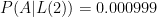
or one in a thousand! So notice that the later I am, the higher the odds that I’m in trouble. Yet, the numbers (admittedly based on the handwaving assumptions above) are small enough for us to not worry!

Bayesian reasoning has its implications elsewhere, too. There is the medical case, as Henderson’s blogpost illustrates. Then we can use this to determine whether a wrong act was due to stupidity or due to malice. And so forth.

But what Henderson’s doctor told him is truly an immortal line:

When you hear hooves, think horses, not zebras.

Narendra Modi and the Correlation Term

In a speech in Canada last night, Prime Minister Narendra Modi said that the relationship between India and Canada is like the “2ab term” in the formula for expansion of (a+b)^2.

Unfortunately for him, this has been widely lampooned on twitter, with some people seemingly not getting the mathematical reference, and others making up some unintended consequences of it.

In my opinion, however, it is a masterstroke, and brings to notice something that people commonly ignore – what I call as the “correlation term”. When any kind of break up or disagreement happens – like someone quitting a job, or a couple breaking up, or a band disbanding, people are bound to ask the question of whose fault it was. The general assumption is that if two entities did not agree, it was because both of them sucked.

However, considering the frequency at which such events (breakups or disagreements ) happen, and that people who are generally “good” are involved in such events, the badness of one of the parties involve simply cannot explain them. So the question arises – if both parties were flawless why did the relationship go wrong? And this is where the correlation term comes in!

It is rather easy to explain using vector calculus. If you have two vectors A and B, the magnitude of the sum of the two vectors is given by \sqrt{|A|^2 + |B|^2 + 2 |A||B| cos \theta} where |A|,|B| are the magnitudes of the two vectors respectively and \theta is the angle between them. It is easy to see from the above formula that the magnitude of the sum of the vectors is dependent not only on the magnitudes of the individual vectors, but also on the angle between them.

To illustrate with some examples, if A and B are perfectly aligned (\theta = 0, cos \theta = 1), then the magnitude of their vector sum is the sum of their magnitudes. If they oppose each other, then the magnitude of their vector sum is the difference of their magnitudes. And if A and B are orthogonal, then cos \theta = 0 or the magnitude of their vector sum is \sqrt{|A|^2 + |B|^2}.

And if we move from vector algebra to statistics, then if A and B represent two datasets, the “cos \theta” is nothing but the correlation between A and B. And in the investing world, correlation is a fairly important and widely used concept!

So essentially, the concept that the Prime Minister alluded to in his lecture in Canada is rather important, and while it is commonly used in both science and finance, it is something people generally disregard in their daily lives. From this point of view, kudos to the Prime Minister for bringing up this concept of the correlation term! And here is my interpretation of it:

At first I was a bit upset with Modi because he only mentioned “2ab” and left out the correlation term (\theta). Thinking about it some more, I reasoned that the reason he left it out was to imply that it was equal to 1, or that the angle between the a and b in this case (i.e. India and Canada’s interests) is zero, or in other words, that India and Canada’s interests are perfectly aligned! There could have been no better way of putting it!

So thanks to the Prime Minister for bringing up this rather important concept of correlation to public notice, and I hope that people start appreciating the nuances of the concept rather than brainlessly lampooning him!

Review: The Theory That Would Not Die

I was introduced to Bayes’ Theorem of Conditional Probabilities in a rather innocuous manner back when I was in Standard 12. KVP Raghavan, our math teacher, talked about pulling black and white balls out of three different boxes. “If you select a box at random, draw two balls and find that both are black, what is the probability you selected box one?” , he asked and explained to us the concept of Bayes’ Theorem. It was intuitive, and I accepted it as truth.

I wouldn’t come across the theorem, however, for another four years or so, until in a course on Communication, I came across a concept called “Hidden Markov Models”. If you were to observe a signal, and it could have come out of four different transmitters, what are the odds that it was generated by transmitter one? Once again, it was rather intuitive. And once again, I wouldn’t come across or use this theorem for a few years.

A couple of years back, I started following the blog of Columbia Statistics and Social Sciences Professor Andrew Gelman. Here, I came across the terms “Bayesian” and “non-Bayesian”. For a long time, the terms baffled me to no end. I just couldn’t get what the big deal about Bayes’ Theorem was – as far as I was concerned it was intuitive and “truth” and saw no reason to disbelieve it. However, Gelman frequently allured to this topic, and started using the term “frequentists” for non-Bayesians. It was puzzling as to why people refused to accept such an intuitive rule.

The Theory That Would Not Die is Shannon Bertsch McGrayne’s attempt to tell the history of the Bayes’ Theorem. The theorem, according to McGrayne,

survived five near-fatal blows: Bayes had shelved it; Price published it but was ignored; Laplace discovered his own version but later favored his frequency theory; frequentists virstually banned it; and the military kept it secret.

The book is about the development of the theorem and associated methods over the last two hundred and fifty years, ever since Rev. Thomas Bayes first came up with it. It talks about the controversies associated with the theorem, about people who supported, revived or opposed it; about key applications of the theorem, and about how it was frequently and for long periods virtually ostracized.

While the book is ostensibly about Bayes’s Theorem, it is also a story of how science develops, and comes to be. Bayes proposed his theorem but didn’t publish it. His friend Price put things together and published it but without any impact. Laplace independently discovered it, but later in his life moved away from it, using frequency-based methods instead. The French army revived it and used it to determine the most optimal way to fire artillery shells. But then academic statisticians shunned it and “Bayes” became a swearword in academic circles. Once again, it saw a revival at the Second World War, helping break codes and test weapons, but all this work was classified. And then it found supporters in unlikely places – biology departments, Harvard Business School and military labs, but statistics departments continued to oppose.

The above story is pretty representative of how a theory develops – initially it finds few takers. Then popularity grows, but the establishment doesn’t like it. It then finds support from unusual places. Soon, this support comes from enough places to build momentum. The establishment continues to oppose but is then bypassed. Soon everyone accepts it, but some doubters remain..

Coming back to Bayes’ Theorem – why is it controversial and why was it ostracized for long periods of time? Fundamentally it has to do with the definition of probability. According to “frequentists”, who should more correctly be called “objectivists”, probability is objective, and based on counting. Objectivists believe that probability is based on observation and data alone, and not from subjective beliefs. If you ask an objectivist, for example, the probability of rain in Bangalore tomorrow, he will be unable to give you an answer – “rain in Bangalore tomorrow” is not a repeatable event, and cannot be observed multiple times in order to build a model.

Bayesians, who should be more correctly be called “subjectivists”, on the other hand believe that probability can also come from subjective beliefs. So it is possible to infer the probability of rain in Bangalore tomorrow based on other factors – like the cloud cover in Bangalore today or today’s maximum temperature. According to subjectivists (which is the current prevailing thought), probability for one-time events is also defined, and can be inferred from other subjective factors.

Essentially, the the battle between Bayesians and frequentists is more to do with the definition of probability than with whether it makes sense to define inverse probabilities as in Bayes’ Theorem. The theorem is controversial only because the prevailing statistical establishment did not agree with the “subjectivist” definition of probability.

There are some books that I call as ‘blog-books’. These usually contain ideas that could be easily explained in a blog post, but is expanded into book length – possibly because it is easier to monetize a book-length manuscript than a blog-length one. When I first downloaded a sample of this book to my Kindle I was apprehensive that this book might also fall under that category – after all, how much can you talk about a theorem without getting too technical? However, McGrayne avoids falling into that trap. She peppers the book with interesting stories of the application of Bayes’ Theorem through the years, and also short biographical tidbits of some of the people who helped shape the theorem. Sometimes (especially towards the end) some of these examples (of applications) seem a bit laboured, but overall, the books sustains adequate interest from the reader through its length.

If I had one quibble with the book, it would be that even after the descriptions of the story of the theorem, the book talks about “Bayesian” and ‘non-Bayesian” camps, and talk about certain scientists “not doing enough to further the Bayesian cause”. For someone who is primarily interested in getting information out of data, and doesn’t care about the methods involved, it was a bit grating that scientists be graded on their “contribution to the Bayesian cause” rather than their “contribution to science”. Given the polarizing history of the theorem, however, it is perhaps not that surprising.

The Theory That Would Not Die: How Bayes’ Rule Cracked the Enigma Code, Hunted Down Russian Submarines, and Emerged Triumphant from Two Centuries of Controversy
by Sharon Bertsch McGrayne
U
SD 12.27 (Kindle edition)
360 pages (including appendices and notes)

Hedgehogs and foxes: Or, a day in the life of a quant

I must state at the outset that this post is inspired by the second chapter of Nate Silver’s book The Signal and the Noise. In that chapter, which is about election forecasting, Silver draws upon the old Russian parable of the hedgehog and the fox. According to that story, the fox knows several tricks while the hedgehog knows only one – curling up into a ball. The story ends in favour of the hedgehog, as none of the tricks of the unfocused fox can help him evade the predator.

Most political pundits, says Silver, are like hedgehogs. They have just one central idea to their punditry and they tend to analyze all issues through that. A good political forecaster, however, needs to be able to accept and process any new data inputs, and include that in his analysis. With just one technique, this can be hard to achieve and so Silver says that to be a good political forecaster one needs to be a fox. While this might lead to some contradictory statements and thus bad punditry, it leads to good forecasts. Anyway, you can know about election forecasting from Silver’s book.

The world of “quant” and “analytics” which I inhabit is again similarly full of hedgehogs. You have the statisticians, whose solution for every problem is a statistical model. They can wax eloquent about Log Likelihood Estimators but can have trouble explaining why you should use that in the first place. Then you have the banking quants (I used to be one of those), who are proficient in derivatives pricing, stochastic calculus and partial differential equations, but if you ask them why a stock price movement is generally assumed to be lognormal, they don’t have answers. Then you have the coders, who can hack, scrape and write really efficient code, but don’t know much math. And mathematicians who can come up with elegant solutions but who are divorced from reality.

While you might make a career out of falling under any of the above categories, to truly unleash your potential as a quant, you should be able to do all. You should be a fox and should know each of these  tricks. And unlike the fox in the Old Russian fairy tale, the key to being a good fox is to know what trick to use when. Let me illustrate this with an example from my work today (actual problem statement masked since it involves client information).

So there were two possible distributions that a particular data point could have come from and I had to try and analyze which of them it came from (simple Bayesian probability, you might think). However, calculating the probability wasn’t so straightforward, as it wasn’t a standard function. Then I figured I could solve the probability problem using the inclusion-exclusion principle (maths again), and wrote down a mathematical formulation for it.

Now, I was dealing with a rather large data set, so I would have to use the computer, so I turned my mathematical solution into pseudo-code. Then, I realized that the pseudo-code was recursive, and given the size of the problem I would soon run out of memory. I had to figure out a solution using dynamic programming. Then, following some more code optimization, I had the probability. And then I had to go back to do the Bayesian analysis in order to complete the solution. And then present the solution in the form of a “business solution”, with all the above mathematical jugglery being abstracted from the client.

This versatility can come in handy in other places, too. There was a problem for which I figured out that the appropriate solution involved building a classification tree. However, given the nature of the data at hand, none of the off-the-shelf classification tree algorithms for were ideal. So I simply went ahead and wrote my own code for creating such trees. Then, I figured that classification trees are in effect a greedy algorithm, and can lead to getting stuck at local optima. And so I put in a simulated annealing aspect to it.

While I may not have in depth knowledge of any of the above techniques (to gain breadth you have to sacrifice depth), that I’m aware of a wide variety of techniques means I can provide the solution that is best for the problem at hand. And as I go along, I hope to keep learning more and more techniques – even if I don’t use them, being aware of them will lead to better overall problem solving.