Recreating Tufte, and Bangalore weather

For most of my life, I pretty much haven’t understood what the point of “recreating” is. For example, in school if someone says they were going to “act out ______’s _____” I would wonder what the point of it was – that story is well known so they might as well do something more creative.

Later on in life, maybe some 12-13 years back, I discovered the joy in “retelling known stories” – since everyone knows the story you can be far more expressive in how you tell it. Still, however, just “re-creation” (not recreation) never really fascinated me. Most of the point of doing things is to do them your way, I’ve believed (and nowadays, if you think of it, most re-creating can be outsourced to a generative AI).

And the this weekend that changed. On Saturday, I made the long-pending trip to Blossom (helped that daughter had a birthday party to attend nearby), and among other things, I bought Edward Tufte’s classic “The Visual Display of Quantitative Information“. I had read a pirated PDF of this a decade ago (when I was starting out in “data science”), but always wanted the “real thing”.

And this physical copy, designed by Tufte himself, is an absolute joy to read. And I’m paying more attention to the (really beautiful) graphics. So, when I came across this chart of New York weather, I knew I had to recreate it.

A few months earlier, I had dowloaded the dataset for Bangalore’s hourly temperature and rainfall since 1981 (i.e. a bit longer than my own life). This dataset ended in November 2022, but I wasn’t concerned. Basically, this is such a large and complex dataset that so far I had been unable to come up with an easy way to visualise it. So, when I saw this thing from Tufte, recreating would be a good idea.

I spent about an hour and half yesterday doing this. I’ve ignored the colour schemes and other “aesthetic” stuff (just realised I’ve not included the right axis in my re-creation). But I do think I’ve got something fairly good.

My re-creation of Tufte’s New York weather map, in the context of Bangalore in 2022

2022 was an unusual weather year for Bangalore and it shows in this graph. May wasn’t as hot as usual, and there were some rather cold days. Bangalore recorded its coldest October and November days since the 90s (though as this graph shows, not a record by any means). It was overall a really wet year, constantly raining from May to November. The graph shows all of it.

Also if you look at the “noraml pattern” and the records, you see Bangalore’s unusual climate (yes, I do mean “climate” and not “weather” here). Thanks to the monsoons (and pre-monsoons), April is the hottest month. Summer, this year, has already started – in the afternoons it is impossible to go out now. The minimum temperatures are remarkably consistent through the year (so except early in the mornings, you pretty much NEVER need a sweater here – at least I haven’t after I moved back from London).

There is so much more I can do. I’m glad to have come across a template to analyse the data using. Whenever I get the enthu (you know what this website is called) I’ll upload my code to produce this graph onto github or something. And when I get more enthu, I’ll make it aesthetically similar to Tufte’s graph (and include December 2022 data as well).


Placing data labels in bar graphs

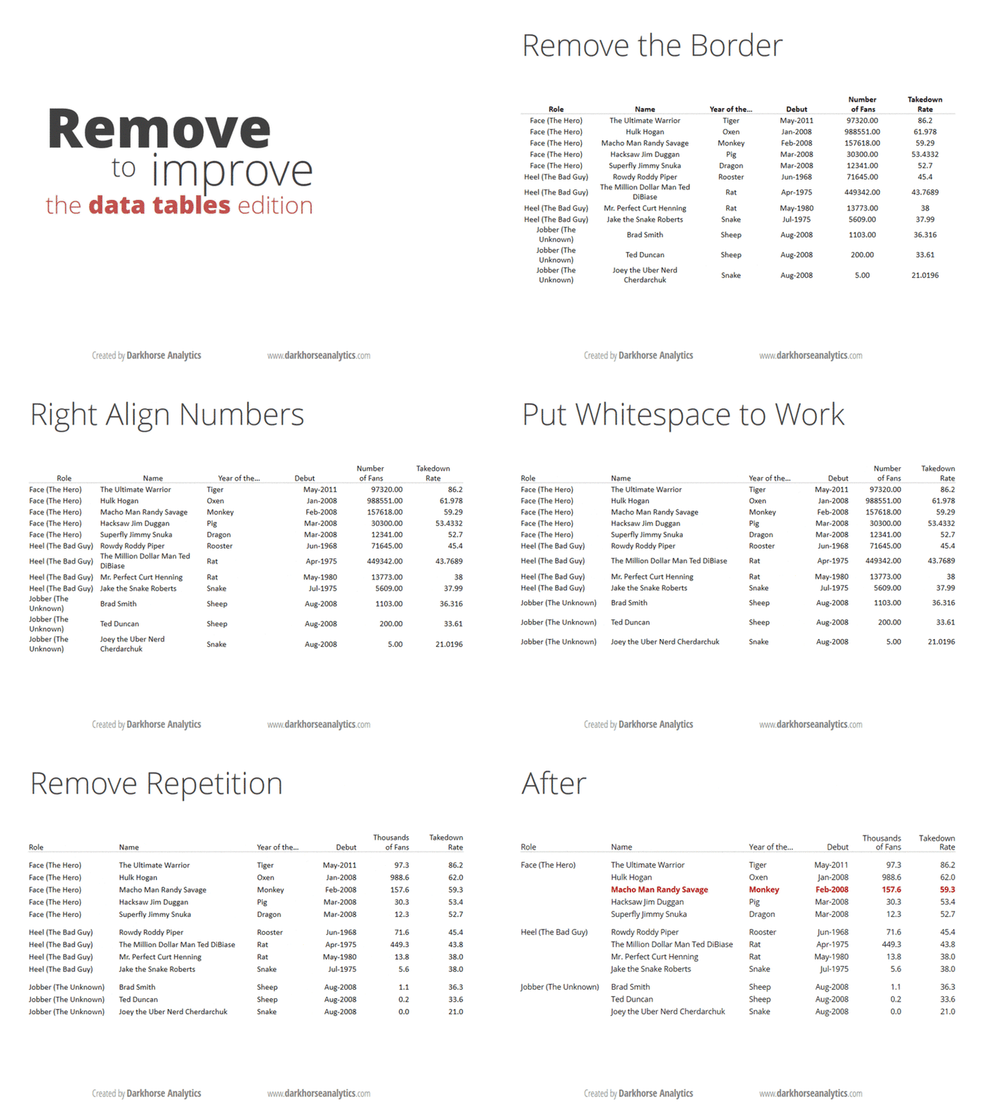
If you think you’re a data visualisation junkie, it’s likely that you’ve read Edward Tufte’s Visual Display Of Quantitative Information. If you are only a casual observer of the topic, you are likely to have come across these gifs that show you how to clean up a bar graph and a data table.

And if you are a real geek when it comes to visualisation, and you are the sort of person who likes long-form articles about the information technology industry, I’m sure you’ve come across Eugene Wei’s massive essay on “remove the legend to become one“.

The idea in the last one is that when you have something like a line graph, a legend telling you which line represents what can be distracting, especially if you have too many lines. You need to constantly move your head back and forth between the chart and the table as you try to interpret it. So, Wei says, in order to “become a legend” (by presenting information that is easily consumable), you need to remove the legend.

My equivalent of that for bar graphs is to put data labels directly on the bar, rather than having the reader keep looking at a scale (the above gif with bar graphs also does this). It makes for easier reading, and by definition, the bar graph conveys the information on the relative sizes of the different data points as well.

There is one problem, though, especially when you’re drawing what my daughter calls “sleeping bar graphs” (horizontal) – where do you really put the text so that it is easily visible? This becomes especially important if you’re using a package like R ggplot where you have control over where to place the text, what size to use and so on.

The basic question is – do you place the label inside or outside the bar? I was grappling with this question yesterday while making some client chart. When I placed the labels inside the bar, I found that some of the labels couldn’t be displayed in full when the bars were too short. And since these were bars that were being generated programmatically, I had no clue beforehand how long the bars would be.

So I decided to put all the labels outside. This presented a different problem – with the long bars. The graph would automatically get cut off a little after the longest bar ended, so if you placed the text outside, then the labels on the longest bar couldn’t be seen! Again the graphs have to come out programmatically so when you’re making them you don’t know what the length of the longest bar will be.

I finally settled on this middle ground – if the bar is at least half as long as the longest bar in the chart set, then you put the label inside the bar. If the bar is shorter than half the longest bar, then you put the label outside the bar. And then, the text inside the bar is right-justified (so it ends just inside the end of the bar), and the text outside the bar is left-justified (so it starts exactly where the bar ends). And ggplot gives you enough flexibility to decide the justification (‘hjust’) and colour of the text (I keep it white if it is inside the bar, black if outside), that the whole thing can be done programmatically, while producing nice and easy-to-understand bar graphs with nice labels.

Obviously I can’t share my client charts here, but here is one I made for the doubling days for covid-19 cases by district in India. I mean it’s not exactly what I said here, but comes close (the manual element here is a bit more).