mathematics – Page 3 – Pertinent Observations

Deranging groups

Ok so this is a mathematical problem. I plan to give three group assignments to my IIMB class. Let’s assume that there are 60 kids and for each assignment I want them to form groups of four members each. For the first assignment I’ve let them form the groups themselves.

For the second assignment, though, I want to create a “derangement” of these groups – in the sense that I want to form a different set of 15 groups of 4 members each such that no pair of students who are in the same group for assignment 1 will be in the same group for assignment 2. And I’m looking for an algorithm to thus “derange” my students. And whether it is possible at all to derange students thus.

My inclination is that this might have a solution in graph theory – in terms of graph colouring or something? Take the students from the first group and join every pair of students that are in the same group with an edge. Then colour the nodes of the graph. Pick nodes of the same colour (these are students that haven’t been in groups together) and randomly assign them to new groups. Repeat for all colours.

Question is how many colours we need to colour the graph. If it’s planar, we’ll need only 4 colours! And considering that the first assignment has 4 students per group, the maximum degree of a node is 3. If the maximum degree of an edge is 3, does that say anything about the planarity of the graph? If I derange the students once for assignment 2, can I do it again for assignment 3 (now each node has a degree of 6!) ? How do I think about this mathematically? Can you help?

Factorising 2015

Sometimes when I come across a new number I factorise it, just for kicks. So when the year ticked over that’s what I tried doing.

It is intuitive that 2015 is divisible by 5, so I quickly decomposed it into 5 times 403. And then my intuitive reaction was “403 looks prime. So 2015 is such an uninteresting number”.

But then doing the rigorous analysis (dividing 403 by all primes <= 20 (= sqrt (403)), I figured that it goes by 13, and can be decomposed into 13 and 31, which makes it quite interesting!

So 2015 is a product of 5, 13 and 31, which makes it interesting, in that it is a product of relatively small primes!

The year began well here in Bangalore. It started drizzling soon after the clocks ticked over 12, and this morning has also been what people might describe as “gloomy” but what I find to be absolutely romantic weather!

Wish you all a happy and prosperous 2015!

Why standard deviation is not a good measure of volatility

Most finance textbooks, at least the ones that are popular in Business Schools, use standard deviation as a measure of volatility of a stock price. In this post, we will examine why it is not a great idea. To put it in one line, the use of standard deviation loses information on the ordering of the price movement.

As earlier, let us look at two data sets and try to measure their volatility. Let us consider two time series (let’s simply call them “series1” and “series2”) and try and compare their volatilities. The table here shows the two series:

What can you say of the two series now? You think they are similar? You might notice that both contain the same set of numbers, but jumbled up. Let us look at the volatility as expressed by standard deviation. Unsurprisingly, since both series contain the same set of numbers, the volatility of both series is identical – at 8.655.

However, does this mean that the two series are equally volatile? Not particularly, as you can see from this graph of the two series:

It is clear from the graph (if it was not clear from the table already) that Series 2 is much more volatile than series 1. So how can we measure it? Most textbooks on quantitative finance (as opposed to textbooks on finance) use “Quadratic Variation” as a measure of volatility. How do we measure quadratic variation?

If we have a series of numbers from $a_1$ to $a_n$ , then the quadratic variation of this series is measured as

$sum_{i=2 to n} (a_i - a_{i-1})^2$

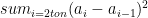
Notice that the primary difference feature of the quadratic variation is that it takes into account the sequence. So when you have something like series 2, with alternating positive and negative jumps, it gets captured in the quadratic variation. So what would be the quadratic variation values for the two time series we have here?

The QV of series 1 is 29 while that of series 2 is a whopping 6119, which is probably a fair indicator of their relative volatilities.

So why standard deviation?

Now you might ask why textbooks use standard deviation at all then, if it misses out so much of the variation. The answer, not surprisingly, lies in quantitative finance. When the price of a stock (X) is governed by a Wiener process, or

$dX = sigma dW$

then the quadratic variation of the stock price (between time 0 and time t) can be shown to be $sigma^2 t$ , which for t = 1 is $sigma^2$ which is the variance of the process.

Because for a particular kind of process, which is commonly used to model stock price movement, the quadratic variation is equal to variance, variance is commonly used as a substitute for quadratic variation as a measure of volatility.

However, considering that in practice stock prices are seldom Brownian (either arithmetic or geometric), this equivalence doesn’t necessarily hold.

This is also a point that Benoit Mandelbrot makes in his excellent book The (mis)Behaviour of Markets. He calls this the Joseph effect (he uses the biblical story of Joseph, who dreamt of seven fat cows being eaten by seven lean foxes, and predicted that seven years of Nile floods would be followed by seven years of drought). Financial analysts, by using a simple variance (or standard deviation) to characterize volatility, miss out on such serial effects.